Mapping regional runout susceptibility from predicted source areas

The runoptGPP package was developed for automatic parameter selection for single event and regional runout modeling using the random walk and PCM components of the Gravitational Process Path (GPP) Model tool in SAGA-GIS. The optimization procedure uses a two-stage approach, where we first optimize the random walk model to find the ‘best’ simulation of runout path, and then plug-in these values to the PCM model to optimize for runout distance. The performance of the runout path is based on the area under the receiver operating characteristic curve (AUROC), and runout distance is based on a measure of relative error.

This vignette

Provides an example of regionally mapping debris flow runout from predicted source areas

Load packages and data

In this example, we apply an optimized runout model to a sub catchment of our study area. First, the required packages and data are loaded, data is cropped by a sub catchment boundary, and we create a hillshade model for improving visualization of our results.

library(runoptGPP)
library(raster)
library(rgdal)
library(Rsagacmd)
library(ggplot2) # Plotting maps
library(patchwork) # Tile multiple maps together
library(ggnewscale) # Allow multiple scales in a map

# Initiate a SAGA-GIS geoprocessing object
saga <- saga_gis(opt_lib = "sim_geomorphology")

# Load shapefile of sub catchment polygons
sub_catchments <- readOGR("sub_catchments.shp")

#> OGR data source with driver: ESRI Shapefile 
#> Source: "/home/jason/Data/Chile/sub_catchments.shp", layer: "sub_catchments"
#> with 58 features
#> It has 15 fields
#> Integer64 fields read as strings:  OBJECTID ID No elev_min elev_max elev_media elev_rango pend_min pend_max pend_media pend_rango Seleccion

# Load and crop DEM for a single sub catchment
dem <- raster("elev_alos_12_5m.tif")
dem <- crop(dem, sub_catchments[sub_catchments$ID == 56,])
dem <- mask(dem, sub_catchments[sub_catchments$ID == 56,])

# Load and crop source area prediction raster
source_pred <- raster("source_pred_gam.tif")
source_pred <- crop(source_pred, sub_catchments[sub_catchments$ID == 56,])
source_pred <- mask(source_pred, sub_catchments[sub_catchments$ID == 56,])

# For visualization make a hillshade model from the DEM
slope <- terrain(dem, opt='slope')
aspect <- terrain(dem, opt='aspect')
hillshade <- hillShade(slope, aspect, angle=40, direction=270)

Classify source prediction probabilities

We need to define a probability threshold to classify a source area prediction grid cell (values range from 0 to 1) as a source area.

# Aggregate data for quicker mapping
hillshade_agg <- aggregate(hillshade, fact = 5, fun = mean)
source_agg <- aggregate(source_pred, fact = 5, fun = mean)

# Transform raster data into a data frame for use with ggplot
hillshade_df <- as.data.frame(hillshade_agg, xy = TRUE)
hillshade_df <- hillshade_df[!is.na(hillshade_df[,3]),]

source_df <- as.data.frame(source_agg, xy = TRUE)
source_df <- source_df[!is.na(source_df[,3]),]
names(source_df) <- c("x", "y", "pred")

# Create source area prediction map
map.srcpred <- ggplot() +
  geom_tile(data=hillshade_df, aes(x=x, y=y, fill = layer),
              show.legend = FALSE) +
  scale_fill_gradient(high = "white", low = "black", na.value = "#FFFFFF") +
  new_scale("fill") +
  geom_tile(data=source_df, aes(x=x, y=y, fill = pred) ) +
  scale_fill_viridis_c(name = "Source area\nprediction",  alpha = 0.6, direction = -1) +
  xlab("Easting (m)") +
  ylab("Northing (m)") +
  coord_fixed() +
  theme_light() +
  theme(text = element_text(size = 9), axis.title = element_text(size = 9),
        axis.text = element_text(size = 6), axis.text.y = element_text(angle = 90))
map.srcpred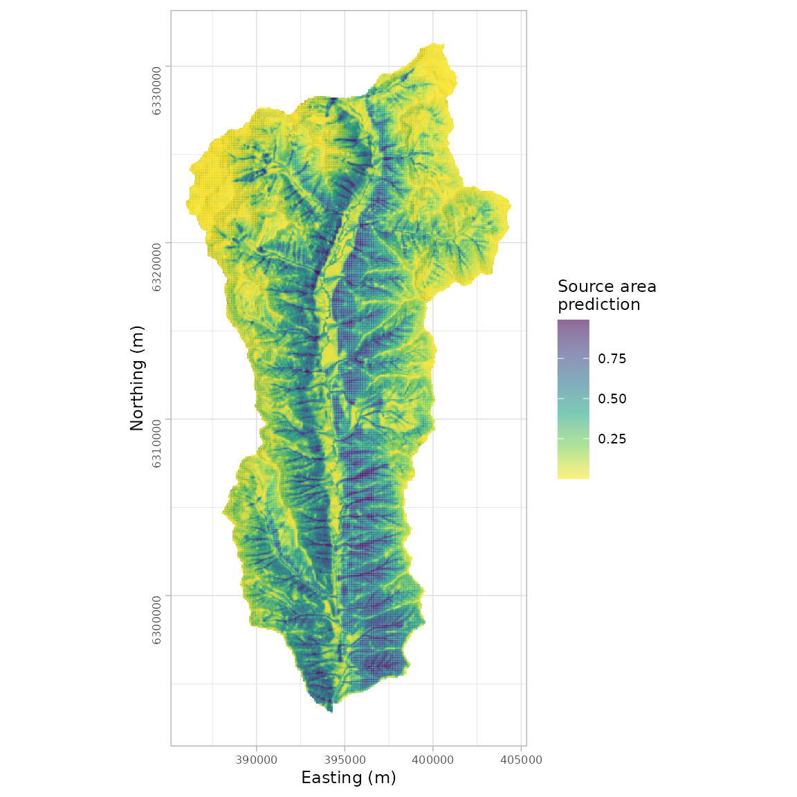

In this example, we will use a threshold of 0.7. The rasterThreshold function allows use to easily reclassify our source area prediction map.

source_area <- rasterThreshold(source_pred, c(0.7, Inf))

# Again aggregate data for quicker mapping
sourcearea_agg <- aggregate(source_area, fact = 5, fun = mean)
sourcearea_df <- as.data.frame(sourcearea_agg, xy = TRUE)
sourcearea_df <- sourcearea_df[!is.na(sourcearea_df[,3]),]
names(sourcearea_df) <- c("x", "y", "pred")

# Create classified source area map
map.srcarea <- ggplot() +
  geom_tile(data=hillshade_df, aes(x=x, y=y, fill = layer),
              show.legend = FALSE) +
  scale_fill_gradient(high = "white", low = "black", na.value = "#FFFFFF") +
  new_scale("fill") +
  geom_tile(data=sourcearea_df, alpha = 0.6, aes(x=x, y=y, fill = "") ) +
  scale_fill_manual(name = "Source area", values = "#e74c3c" ) +
  xlab("Easting (m)") +
  ylab("Northing (m)") +
  coord_fixed() +
  theme_light() +
  theme(text = element_text(size = 9), axis.title = element_text(size = 9),
        axis.text = element_text(size = 6), axis.text.y = element_text(angle = 90))
map.srcarea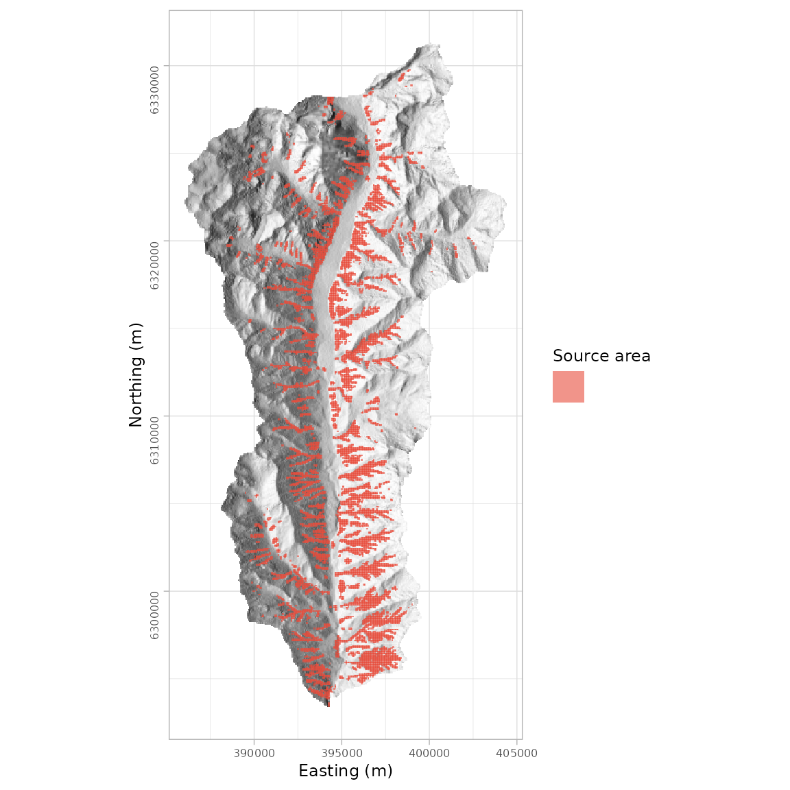

Apply runout model to reclassified source area prediction

Rsagacmd can be used to access the GPP model from SAGA-GIS and simulate runout using the reclassified source areas from R. We can plug-in our regionally optimized random walk and PCM model parameters.

gpp <- saga$sim_geomorphology$gravitational_process_path_model(dem = dem, 
                                                               release_areas = source_area,
                                                               process_path_model = 1,
                                                               rw_slope_thres = 40,
                                                               rw_exponent = 3,
                                                               rw_persistence = 1.9,
                                                               gpp_iterations = 1000,
                                                               friction_model = 5,
                                                               friction_mu = 0.11,
                                                               friction_mass_to_drag = 40)

# Save/Export GPP simulation rasters
writeRaster(gpp$process_area, filename="gpp_process_area.tif", format = "GTiff")
writeRaster(gpp$max_velocity, filename="gpp_max_velocity.tif", format = "GTiff")
writeRaster(gpp$stop_positions, filename="gpp_stop_positions.tif", format = "GTiff")

# Load exported rasters
parea <- raster("gpp_process_area.tif")
maxvel <- raster("gpp_max_velocity.tif")
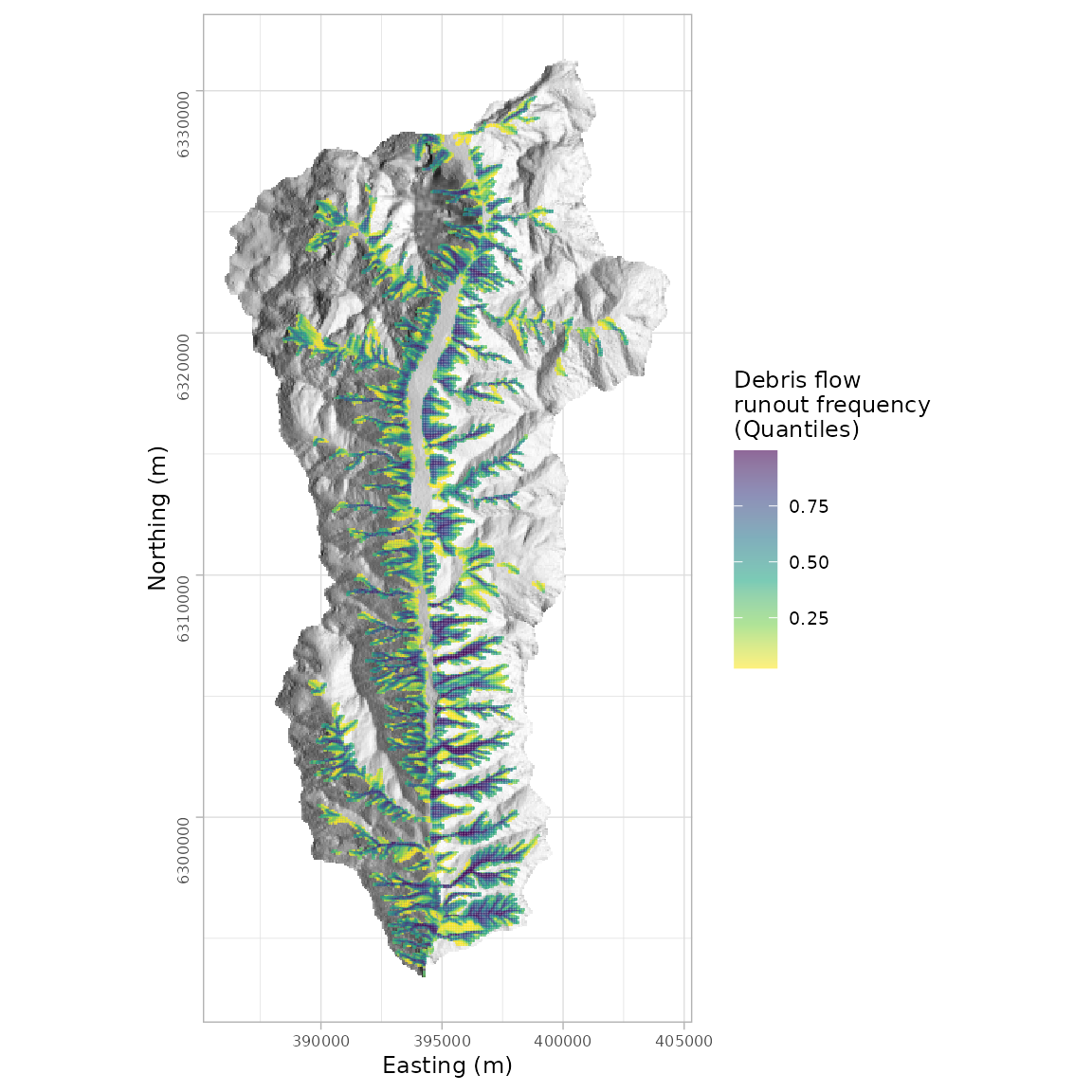
stopp <- raster("gpp_stop_positions.tif")

Now we can map our regional runout modelling results,

# Quantile classification of runout and stop position frequencies
parea_cdf <- rasterCdf(parea)
stopp_cdf <- rasterCdf(stopp)

# Aggregate for quicker mapping
parea_cdf <- aggregate(parea_cdf, fact = 5, fun = mean)

# Format to data frame for ggplot2
parea_df <- as.data.frame(parea_cdf, xy = TRUE)
parea_df <- parea_df[!is.na(parea_df[,3]),]

# Process area map
map.parea <- ggplot() +
  geom_tile(data=hillshade_df, aes(x=x, y=y, fill = layer),
              show.legend = FALSE) +
  scale_fill_gradient(high = "white", low = "black", na.value = "#FFFFFF") +

  new_scale("fill") +
  geom_tile(data=parea_df, aes(x=x, y=y, fill = gpp_process_area) ) +
  scale_fill_viridis_c(name = "Debris flow\nrunout frequency\n(Quantiles)",  alpha = 0.6, direction = -1) +

  xlab("Easting (m)") +
  ylab("Northing (m)") +
  coord_fixed() +
  theme_light() +
  theme(text = element_text(size = 9), axis.title = element_text(size = 9),
        axis.text = element_text(size = 6), axis.text.y = element_text(angle = 90))
map.parea

Jason Goetz

2021-04-12

Load packages and data

Classify source prediction probabilities

Apply runout model to reclassified source area prediction